Assume that you are interested in some attribute or characteristic of a very large number of people, such as the average hours of sleep per night for all undergraduates at all universities. Clearly, you are not going to do this by measuring the hours of sleep for every student, as that would be difficult to impossible. So, instead, you will probably take a relatively small sample of students (e.g., 100 people), ask each of them how many hours of sleep they usually get, and then use these data to estimate the average for all undergraduates.
The process outlined above can be thought of as having three phases or steps: (1) collect a sample, (2) summarize the data in the sample, and (3) use the summarized data to make the estimate of the entire population. The issues related to collecting the sample, such as how one ensures that the sample is representative of the entire population will not be discussed here. Likewise, the way that one uses the summary of a sample to calculate an estimate of the population will not be explained here. This unit will focus on the second step: the way in which psychologists summarize data.
The general label for procedures that summarize data is descriptive statistics. This can be contrasted with procedures that make estimates of population values, which are known as inferential statistics. Thus, descriptive and inferential statistics each give different insights into the nature of the data gathered. Descriptive statistics describe the data so that the big picture can be seen. How? By organizing and summarizing properties of a data set. Calculating descriptive statistics takes unordered observations and logically organizes them in some way. This allow us to describe the data obtained, but it does not make conclusions beyond the sample. This is important, because part of conducting (good) research is being able to communicate your findings to other people, and descriptive statistics will allow you to do this quickly, clearly, and precisely.
To prepare you for what follows, please note two things in advance. First, there are several different ways that we can summarize a large set of data. Most of all: we can use numbers or we can use graphical representations. Furthermore, when the data are numerical, we will have options for several of the summary values that we need to calculate. This may seem confusing at first; hopefully, it soon will make sense. Second, but related to the first, the available options for summarizing data often depend on the type of data that we have collected. For example, numerical data, such as hours of sleep per night, are summarized differently from categorical data, such as favorite flavors of ice-cream.
The key to preventing this from becoming confusing is to keep the function of descriptive statistics in mind: we are trying to summarize a large amount of data in a way that can be communicated quickly, clearly, and precisely. In some cases, a few numbers will do the trick; in other cases, you will need to create a plot of the data.
This unit will only discuss the ways in which a single set of values are summarized. When you collect more than one piece of information from every participant in the sample –e.g., you not only ask them how many hours of sleep they usually get, but also ask them for their favorite flavor of ice-cream– then you can do three things using descriptive statistics: summarized the first set of values (on their own), summarize the second set of values (on their own), and summarize the relationship between the two sets of values. This unit only covers the first two of these three. Different ways to summarize the relationship between two sets of values will be covered in Units 7 and 8.
The most-popular way to summarize a set of numerical data –e.g., hours of sleep per night– is in terms of two or three aspects. One always includes values for the center of the data and the spread of the data; in some cases, the shape of the data is also described. A measure of center is a single value that attempts to describe an entire set of data by identifying the central position within that set of data. The full, formal label for this descriptive statistic is measure of central tendency, but most people simply say “center.” Another label for this is the “average.”
A measure of spread is also a single number, but this one indicates how widely the data are distributed around their center. Another way of saying this is to talk about the “variability” of the data. If all of the individual pieces of data are located close to the center, then the value of spread will be low; if the data are widely distributed, then the value of spread will be high.
What makes this a little bit complicated is that there are multiple ways to mathematically define the center and spread of a set of data. For example, both the mean and the median (discussed in detail below) are valid measures of central tendency. Similarly, both the variance (or standard deviation) and the inter-quartile range (also discussed below) are valid measures of spread. This might suggest that there are at least four combinations of center and spread (i.e., two versions of center crossed with two version of spread), but that isn’t true. The standard measures of center and spread actually come in pairs, such that your choice with regard to one forces you to use a particular option for the other. If you define the center as the mean, for example, then you have to use variance (or standard deviation) for spread; if you define the center as the median, then you have to use the inter-quartile range for spread. Because of this dependency, in what follows we shall discuss the standard measures of center and spread in pairs. When this is finished, we shall mention some of the less popular alternatives and then, finally, turn to the issue of shape.
The mean and variance of a set of numerical values are (technically) the first and second moments of the set of data. Although it is not used very often in psychology, the term “moment” is quite popular in physics, where the first moment is the center of mass and the second moment is rotational inertia (these are very useful concepts when describing how hard it is to throw or spin something). The fact that the mean and variance of a set of numbers are the first and second moments isn’t all that important; the key is that they are based on the same approach to the data, which is why they are one of the standard pairs of measures for describing a set of numerical data.
The mean is the most popular and well known measure of central tendency. It is what most people intend when they use the word “average.” The mean can be calculated for any set of numerical data, discrete or continuous, regardless of units or details. The mean is equal to the sum of all values divided by the number of values. So, if we have n values in a data set and they have values x1, x2, …, xn, the mean is calculated using the following formula:
where is the technical way of writing “add up all of the X values” (i.e., the upper-case, Greek letter [sigma] tells you to calculate the sum of what follows), and n is the number of pieces of data (which is usually referred to as “sample size”). The short-hand for writing the mean of X is (i.e., you put a bar over the symbol, X in this case; it is pronounced “ex bar”). As a simple example, if the values of X are 2, 4, and 7, then = 13, n = 3, and therefore = 4.33 (after rounding to two decimal places).
Before moving forward, note two things about using the mean as the measure of center. First, the mean is rarely one of the actual values from the original set of data. As an extreme example: when the data are discrete (e.g., whole numbers, like the number of siblings), the mean will almost never match any of the specific values, because the mean will almost never be a whole number as well.
Second, an important property of the mean is that it includes and depends on every value in your set of data. If any value in the data set is changed, then the mean will change. In other words, the mean is “sensitive” to all of the data.
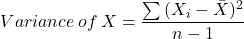
When the center is defined as the mean, the measure of spread to use is the variance (or the square-root of this value, which is the standard deviation). Variance is defined as the average of the squared deviations from the mean. The formula for variance is:
where is the mean (see above). In words, you take each piece of data, subtract the mean, and square the result; do this for each of the n pieces of data and add up the results, then divide by one less than the number of pieces of data. More technically, to determine the variance of a set of scores, you have to 1) find the mean of the scores, 2) compute the deviation scores (the difference between each individual score and the mean), 3) square each of the deviation scores, 4) add up all of the squared deviation scores, and 5) divide by one less than the number of scores. Thus, for example, the variance of 2, 4, and 7 (which have a mean of 4.33, see above) is:
(2 – 4.33) 2 + (4 – 4.33) 2 + (7 – 4.33) 2 = 12.6667
and then divide by (3−1) → 6.33
Note that, because each sub-step of the summation involves a value that has been squared, the value of variance cannot be a negative number. Note, also, that when all of the individual pieces of data are the same, they will all be equal to the mean, so you will be adding up numbers that are all zero, so variance will also be zero. These both make sense, because here we are calculating a measure of how spread out the data are, which will be zero when all of the data are the same and cannot be less than this.
Technically, the value being calculated here is the sample variance, which is different from something known as the population variance. The former is used when we have taken a sample; the latter is used when we have measured every possible value in the entire population. Since we never measure every possible value when doing psychological research, we do not need the formula for population variance and can simply refer to the sample variance as variance.
As mentioned above, some people prefer to express this measure of spread in terms of the square-root of the variance, which is the standard deviation. The main reason for doing this is because the units of variance are the square of the units of the original data, whereas the units of standard deviation are the same as the units of the original data. Thus, for example, if you have response times of 2, 4, and 7 seconds, which have a mean of 4.33 seconds, then the variance is 6.33 seconds 2 (which is difficult to conceptualize), but also have a standard deviation of 2.52 seconds (which is easy to think about).
Conceptually, you can think of the standard deviation as the typical distance of any score from the mean. In other words, the standard deviation represents the standard amount by which individual scores deviate from the mean. The standard deviation uses the mean of the data as a baseline or reference point, and measures variability by considering the distance between each score and the mean.
Note that similar to the mean, both the variance and the standard deviation are sensitive to every value in the set of data; if any one piece of data is changed, then not only will the mean change, but the variance and standard deviation will also be changed.
Let’s calculate now the mean and the standard deviation of the two variables in the following dataset containing the number of study hours before an exam (X, Hours), and the grade obtained in that exam (Y, Grade), for 15 participants. To calculate the mean of Hours, , we sum all of the values for Hours, and divide by the total number of values, 15. To calculate the mean of Grade, , we sum all of the values for Grade, and divide by the total number of values, 15. Doing so, we obtain the mean for Hours ( ) and the mean for Grade ( ). Table 3.1. shows each of the scores, and the deviation scores for each X and Y score. The deviation scores, as explained above, are calculated by subtracting the mean from each of the individual scores.
| Participant | Hours | Grade | ||
| P1 | 8 | 78 | (8 – 13.66) = -5.66 | (78 – 86.46) = -8.46 |
| P2 | 11 | 80 | (11 – 13.66) = -2.66 | (80 – 86.46) = -6.46 |
| P3 | 16 | 89 | (16 – 13.66) = 2.34 | (89 – 86.46) = 2.54 |
| P4 | 14 | 85 | (14 – 13.66) = 0.34 | (85 – 86.46) = -1.46 |
| P5 | 12 | 84 | (12 – 13.66) = -1.66 | (84 – 86.46) = -2.46 |
| P6 | 15 | 86 | (15 – 13.66) = 1.34 | (86 – 86.46) = -0.46 |
| P7 | 18 | 95 | (18 – 13.66) = 4.34 | (95 – 86.46) = 8.54 |
| P8 | 20 | 96 | (20 – 13.66) = 6.34 | (96 – 86.46) = 9.54 |
| P9 | 10 | 83 | (10 – 13.66) = -3.66 | (83 – 86.46) = -3.46 |
| P10 | 9 | 81 | (9 – 13.66) = -4.66 | (81 – 86.46) = -5.46 |
| P11 | 16 | 93 | (16 – 13.66) = 2.34 | (93 – 86.46) = 6.54 |
| P12 | 17 | 92 | (17 – 13.66) = 3.34 | (92 – 86.46) = 5.54 |
| P13 | 13 | 84 | (13 – 13.66) = -0.66 | (84 – 86.46) = -2.46 |
| P14 | 12 | 83 | (12 – 13.66) = -1.66 | (83 – 86.46) = -3.46 |
Table 3.1. Number of study hours before an exam (X, Hours), and the grade obtained in that exam (Y, Grade) for 15 participants. The two most right columns show the deviation scores for each X and Y score.
Once we have the deviation scores for each participant, we square each of the deviation scores, and sum them.
(-5.66) 2 + (-2.66) 2 + (2.34) 2 + (0.34) 2 + (-1.66) 2 + (1.34) 2 + (4.34) 2 + (6.34) 2 + (-3.66) 2 + (-4.66) 2 + …
…( 2.34) 2 + (3.34) 2 + (-0.66) 2 + (-1.66) 2 + (0.34) 2 = 166.334
We then divide that sum by one less than the number of scores, 15 – 1 in this case:
So, 11.66 is the variance for the number of hours in our sample of participants.
In order to obtain the standard deviation, we calculate the square root of the variance:
We follow the same steps to calculate the standard deviation of our participants’ grade. First, we square each of the deviation scores (most right column in Table 3.1), and sum them:
(-8.46) 2 + (-6.46) 2 + (2.54) 2 + (-1.46) 2 + (-2.46) 2 + (-0.46) 2 + (8.54) 2 + (9.54) 2 + (-3.46) 2 + …
… (-5.46) 2 + (6.54) 2 + (5.54) 2 + (-2.46) 2 + (-3.46) 2 + (1.54) 2 = 427.734
Next, we divide that sum by one less than the number of scores, 14:
So, 30.55 is the variance for the grade in our sample of participants.
In order to obtain the standard deviation, we calculate the square root of the variance:
Thus, you can summarize the data in our sample saying that the mean hours of study time are 13.66, with a standard deviation of 3.42, whereas the mean grade is 86.46, with a standard deviation of 5.53.
The second pair of measures for center and spread are based on percentile ranks and percentile values, instead of moments. In general, the percentile rank for a given value is the percent of the data that is smaller (i.e., lower in value). As a simple example, if the data are 2, 4, and 7, then the percentile rank for 5 is 67%, because two of the three values are smaller than 5. Percentile ranks are usually easy to calculate. In contrast, a percentile value (which is kind of the “opposite” of a percentile rank) is much more complicated. For example, the percentile value for 67% when the data are 2, 4, and 7 is something between 4 and 7, because any value between 4 and 7 would be larger than two-thirds of the data. (FYI: the percentile value is this case is 5.02.) Fortunately, we won’t need to worry about the details when calculating that standard measures of center and spread when using the percentile-based method.
The median –which is how the percentile-based method defines center– is best thought of the middle score when the data have been arranged in order of magnitude. To see how this can be done by hand, assume that we start with the data below:
| 65 | 54 | 79 | 57 | 35 | 14 | 56 | 55 | 77 | 45 | 92 |
We first re-arrange these data from smallest to largest:
| 14 | 35 | 45 | 54 | 55 | 56 | 57 | 65 | 77 | 79 | 92 |
The median is the middle of this new set of scores; in this case, the value (i n blue) is 56. This is the middle value because there are 5 scores lower than it and 5 scores higher than it. Finding the median is very easy when you have an odd number of scores.
What happens when you have an even number of scores? What if you had only 10 scores, instead of 11? In this case, you take the middle two scores, and calculate the mean of them. So, if we start with the following data (which are the same as above, with the last one omitted):
| 65 | 54 | 79 | 57 | 35 | 14 | 56 | 55 | 77 | 45 |
We again re-arrange that data from smallest to largest:
| 14 | 35 | 45 | 54 | 55 | 56 | 57 | 65 | 77 | 79 |
And then calculate the mean of the 5th and 6th values (tied for the middle , in blue) to get a median of 55.50.
In general, the median is the value that splits the entire set of data into two equal halves. Because of this, the other name for the median is 50th percentile –50% of the data are below this value and 50% of the data are above this value. This makes the median a reasonable alternative definition of center.
The inter-quartile range (typically named using its initials, IQR) is the measure of spread that is paired with the median as the measure of center. As the name suggests, the IQR divides the data into four sub-sets, instead of just two: the bottom quarter, the next higher quarter, the next higher quarter, and the top quarter (the same as for the median, you must start by re-arranging the data from smallest to largest). As described above, the median is the dividing line between the middle two quarters. The IQR is the distance between the dividing line between the bottom two quarters and the dividing line between the top two quarters.
Technically, the IQR is the distance between the 25th percentile and the 75th percentile. You calculate the value for which 25% of the data is below this point, then you calculate the value for which 25% of the data is above this point, and then you subtract the first from the second. Because the 75th percentile cannot be lower than the 25th percentile (and is almost always much higher), the value for IQR cannot be negative number.
Returning to our example set of 11 values, for which the median was 56, the way that you can calculate the IQR by hand is as follows. First, focus only on those values that are to the left of (i.e., lower than) the middle value:
| 14 | 35 | 45 | 54 | 55 | 56 | 57 | 65 | 77 | 79 | 92 |
Then calculate the “median” of these values. In this case, the answer is 45, because the third box is the middle of these five boxes. Therefore, the 25th percentile is 45.
Next, focus on the values that are to the right of (i.e., higher than) the original median:
| 14 | 35 | 45 | 54 | 55 | 56 | 57 | 65 | 77 | 79 | 92 |
The middle of these values, which is 77, is the 75th percentile. Therefore, the IQR for these data is 32, because 77 – 45 = 32. Note how, when the original set of data has an odd number of values (which made it easy to find the median), the middle value in the data set was ignored when finding the 25th and 75th percentiles. In the above example, the number of values to be examined in each subsequent step was also odd (i.e., 5 each), so we selected the middle value of each subset to get the 25th and 75th percentiles.
If the number of values to be examined in each subsequent step had been even (e.g., if we had started with 9 values, so that 4 values would be used to get the 25th percentile), then the same averaging rule as we use for median would be used: use the average of the two values that tie for being in the middle. For example, if these are the data (which are the first nine values from the original example after being sorted):
| 14 | 35 | 45 | 54 | 55 | 56 | 57 | 65 | 77 |
The median (in blue) is 55, the 25th percentile (the average of the two values in green) is 40, and the 75th percentile (the average of the two values in red) is 61. Therefore, the IQR for these data is 61 – 40 = 21.
A similar procedure is used when you start with an even number of values, but with a few extra complications (these complications are caused by the particular method of calculating percentiles that is typically used in the psychology). The first change to the procedure for calculating IQR is that now every value is included in one of the two sub-steps for getting the 25th and 75th percentile; none are omitted. For example, if we use the same set of 10 values from above (i.e., the original 11 values with the highest omitted), for which the median was 55.50, then here is what we would use in the first sub-step:
| 14 | 35 | 45 | 54 | 55 | 56 | 57 | 65 | 77 | 79 |
In this case, the 25th percentile will be calculated from an odd number of values (5). We start in the same way before, with the middle of these values (in green), which is 45. Then we adjust it by moving the score 25% of the distance towards next lower value, which is 35. The distance between these two values is 2.50 –i.e., (45 – 35) x .25 = 2.50– so the final value for the 25th percentile is 42.50.
The same thing is done for 75th percentile. This time we would start with:
| 14 | 35 | 45 | 54 | 55 | 56 | 57 | 65 | 77 | 79 |
The starting value (in red) of 65 would then be moved 25% of the distance towards the next higher, which is 77, producing a 75th percentile of 68 –i.e., 65 + ((77 – 65) x .25) = 68. Note how we moved the value away from the median in both cases. If we don’t do this –if we used the same simple method as we used when the original set of data had an odd number of values– then we would slightly under-estimate the value of IQR.
Finally, if we start with an even number of pieces of data and also have an even number for each of the sub-steps (e.g., we started with 8 values), then we again have to apply the correction. Whether you have to shift the 25th and 75th percentiles depends on original number of pieces of data, not the number that are used for the subsequent sub-steps. To demonstrate this, here are the first eight values from the original set of data:
| 14 | 35 | 45 | 54 | 55 | 56 | 57 | 65 |
The first step to calculating the 25th percentile is to average the two values (in green) that tied for being in the middle of the lower half of the data; the answer is 40. Then, as above, move this value 25% of the distance away from the median –i.e., move it down by 2.50, because (45 – 35) x .25 = 2.50. The final value is 37.50.
Then do the same for the upper half of the data:
| 14 | 35 | 45 | 54 | 55 | 56 | 57 | 65 |
Start with the average of the two values (in red) that tied for being in the middle and then shift this value 25% of their difference away from the center. The mean of the two values is 56.50 and after shifting the 75th percentile is 56.75. Thus, the IQR for these eight pieces of data is 56.75 – 37.50 = 19.25.
Note the following about the median and IQR: because these are both based on percentiles, they are not always sensitive to every value in the set of data. Look again at the original set of 11 values used in the examples. Now imagine that the first (lowest) value was 4, instead of 14. Would either the median or the IQR change? The answer is No, neither would change. Now imagine that the last (highest) value was 420, instead of 92. Would either the median or IQR change? Again, the answer is No.
Some of the other values can also change without altering the median and/or IQR, but not all of them. If you changed the 56 in the original set to being 50, instead, for example, then the median would drop from 56 to 55, but the IQR would remain 32. In contrast, if you only changed the 45 to being a 50, then the IQR would drop from 32 to 27, but the median would remain 56.
The one thing that is highly consistent is how you can decrease the lowest value and/or increase the highest value without changing either the median or IQR (as long as you start with at least 5 pieces of data). This is an important property of percentiles-based methods: they are relatively insensitive to the most extreme values. This is quite different from moments-based methods; the mean and variance of a set of data are both sensitive to every value.
Although a vast majority of psychologists use either the mean and variance (as a pair) or the median and IQR (as a pair) as their measures of center and spread, occasionally you might come across a few other options.
The mode is a (rarely-used) way of defining the center of a set of data. The mode is simply the value that appears the most often in a set of data. For example, if your data are 2, 3, 3, 4, 5, and 9, then the mode is 3 because there are two 3s in the data and no other value appears more than once. When you think about other sets of example data, you will probably see why the mode is not very popular. First, many sets of data do not have a meaningful mode. For the set of 2, 4, and 7, all three different values appear once each, so no value is more frequent than any other value. When the data are continuous and measured precisely (e.g., response time in milliseconds), then this problem will happen quite often. Now consider the set of 2, 3, 3, 4, 5, 5, 7, and 9; these data have two modes: 3 and 5. This also happens quite often, especially when the data are discrete, such as when they must all be whole numbers.
But the greatest problem with using the mode as the measure of center is that it is often at one of the extremes, instead of being anywhere near the middle. Here is a favorite example (even if it is not from psychology): the amount of federal income tax paid. The most-frequent value for this –i.e., the mode of federal income tax paid– is zero. This also happens to be the same as the lowest value. In contrast, in 2021, for example, the mean amount of federal income tax paid was a little bit over $10,000.
Another descriptive statistic that you might come across is the range of the data. Sometimes this is given as the lowest and highest values –e.g., “the participant ages ranged from 18 to 24 years”– which provides some information about center and spread simultaneously. Other times the range is more specifically intended as only a measure of spread, so the difference between the highest and lowest values is given –e.g., “the average age was 21 years with a range of 6 years.” There is nothing inherently wrong with providing the range, but it is probably best used as a supplement to one of the pairs of measures for center and spread. This is true because range (in either format) often fails to provide sufficient detail. For example, the set of 18, 18, 18, 18, and 24 and the set of 18, 24, 24, 24, and 24 both range from 18 to 24 (or have a range of 6), even though the data sets are clearly quite different.
When it comes to deciding which measures to use for center and spread when describing a set of numerical data –which is almost always a choice between mean and variance (or standard deviation) or median and IQR– the first thing to keep in mind is that this is not a question of “which is better?”; it is a question of which is more appropriate for the situation. That is, the mean and the median are not just alternative ways of calculating a value for the center of a set of data; they use different definitions of the meaning of center.
So how should you make this decision? One factor that you should consider focuses on a key difference between moments and percentiles that was mentioned above: how the mean and variance of a set of data both depend on every value, whereas the median and IQR are often unaffected by the specific values at the upper and lower extremes. Therefore, if you believe that every value in the set of data is equally important and equally representative of whatever is being studied, then you should probably use the mean and variance for your descriptive statistics. In contrast, if you believe that some extreme values might be outliers (e.g., the participant wasn’t taking the study very seriously or was making random fast guesses), then you might want to use the median and IQR instead.
Another related factor to consider is the shape of the distribution of values in the set of data. If the values are spread around the center in a roughly symmetrical manner, then the mean and the median will be very similar, but if there are more extreme values in one tail of the distribution (e.g., there are more extreme values above the middle than below), this will pull the mean away from the median, and the latter might better match what you think of as the center.
Finally, if you are calculating descriptive statistics as part of a process that will later involve making inferences about the population from which the sample was taken, you might want to consider the type of statistics that you will be using later. Many inferential statistics (including t-tests, ANOVA, and the standard form of the correlation coefficient) are based on moments so, if you plan to use these later, it would be probably more appropriate to summarize the data in terms of mean and variance (or standard deviation). Other statistics (including sign tests and alternative forms of the correlation coefficient) are based on percentiles, so if you plan to use these instead, then the median and IQR might be more appropriate for the descriptive statistics.
Hybrid Methods
Although relatively rare, there is one alternative to making a firm decision between moments (i.e., mean and variance) and percentiles (i.e., median and IQR) –namely, hybrid methods. One example of this is as follows. First, sort the data from smallest to largest (in the same manner as when using percentiles). Then remove a certain number of values from the beginning and end of the list. The most popular version of this is to remove the lowest 2.5% and the highest 2.5% of the data; for example, if you started with 200 pieces of data, remove the first 5 and the last 5, keeping the middle 190. Then switch methods and calculate the mean and variance of the retained data. This method is trying to have the best of both worlds: it is avoiding outliers by removing the extreme values, but it is remaining sensitive to all the data that are being retained. When this method is used, the correct label for the final two values are the “trimmed mean” and “trimmed variance.”
As the name suggests, the shape of a set of data is best thought about in terms of how the data would look if you made some sort of figure or plot of the values. The most popular way to make a plot of a single set of numerical values starts by putting all of the data into something that is called a frequency table. In brief, a frequency table is a list of all possible values, along with how many times each value occurs in the set of data. This is easy to create when there are not very many different values (e.g., number of siblings); it becomes more complicated when almost every value in the set of data is unique (e.g., response time in milliseconds).
The key to resolving the problem of having too many unique values is to “bin” the data. To bin a set of data, you choose a set of equally-spaced cut-offs, which will determine the borders of adjacent bins. For example, if you are working with response times which happen to range from about 300 to 600 milliseconds (with every specific value being unique), you might decide to use bins that are 50 milliseconds wide, such that all values from 301 to 350 go in the first bin, all values from 351 to 400 go in the second bin, etc. Most spreadsheet-based software packages (e.g., Excel) have built-in procedures to do this for you.
As an illustration of this process, let’s go back to the set of 11 values we have used in previous examples:
| 65 | 55 | 79 | 56 | 35 | 14 | 56 | 55 | 77 | 45 | 92 |
Based on the total number of values and their range, we decide to use bins that are 20 units wide. Here are the same data in a frequency table:
| Bin | 1-20 | 21-40 | 41-60 | 61-80 | 81-100 |
| Frequency | 1 | 1 | 5 | 3 | 1 |
Once you have a list of values or bins and the number of pieces of data in each, you can make a frequency histogram of the data, as shown in Figure 3.1:
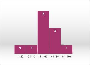
Based on this histogram, we can start to make descriptive statements about the shape of the data. In general, these will concern two aspects, known as skewness and kurtosis, as we shall see next.
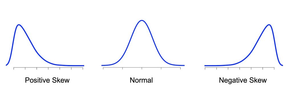
Skewness refers to the lack of symmetry. It the left and right sides of the plot are mirror images of each other, then the distribution has no skew, because it is symmetrical; this is the case of the normal distribution (see Figure 3.2). This clearly is not true for the example in Figure 3.1. If the distribution has a longer tail on the left side, as is true here, then the data are said to have negative skew. If the distribution has a longer “tail” on the right, then the distribution is said to have positive skew. Note that you need to focus on the skinny part of each end of the plot. The example in Figure 3.1 might appear to be heavier on the right, but skew is determined by the length of the skinny tails, which is clearly much longer on the left. As a reference, Figure 3.2. shows you a normal distribution, perfectly symmetrical, so its skewness is zero; to the left and to the right, you can see two skewed distributions, positive and negative. Most of the data points in the distribution with a positive skew have low values, and has a long tail on its right side. The opposite is true for the distribution with negative skew: most of its data points have high values, and has a long tail on its left side.
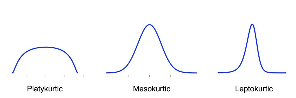
The other aspect of shape, kurtosis, is a bit more complicated. In general, kurtosis refers to how sharply the data are peaked, and is established in reference to a baseline or standard shape, the normal distribution, that has kurtosis zero. When we have a nearly flat distribution, for example when every value occurs equally often, the kurtosis is negative. When the distribution is very pointy, the kurtosis is positive.
If the shape of your data looks like a bell curve, then it’s said to be mesokurtic (“meso” means middle or intermediate in Greek). If the shape of your data is flatter than this, then it’s said to be platykurtic (“platy” means flat in Greek). If your shape is more pointed from this, then your data are leptokurtic (“lepto” means thin, narrow, or pointed in Greek). Examples of these shapes can be seen in Figure 3.3.
Both skew and kurtosis can vary a lot; these two attributes of shape are not completely independent. That is, it is impossible for a perfectly flat distribution to have any skew; it is also impossible for a highly-skewed distribution to have zero kurtosis. A large proportion of the data that is collected by psychologists is approximately normal, but with a long right tail. In this situation, a good verbal label for the overall shape could be positively-skewed normal, even if that seems a bit contradictory, because the true normal distribution is actually symmetrical (see Figures 3.2 and 3.3). The goal is to summarize the shape in a way that is easy to understand while being as accurate as possible. You can always show a picture of your distribution to your audience. A simple summary of the shape of the histogram in Figure 3.1 could be: roughly normal, but with a lot of negative skew; this tells your audience that the data have a decent-sized peak in the middle, but the lower tail is a lot longer than the upper tail.
Numerical Values for Skew and Kurtosis
In some rare situations, you might want to be even more precise about the shape of a set of data. Assuming that you used the mean and variance as your measures of center and spread, in these cases, you can use some (complicated) formulae to calculate specific numerical values for skew and kurtosis. These are the third and fourth moments of the distribution (which is why they can only be used with the mean and variance, because those are the first and second moments of the data). The details of these measures are beyond this course, but to give you an idea, as indicated above, values that depart from zero tells you that the shape is different from the normal distribution. A value of skew that is less than –1 or greater than +1 implies that the shape is notably skewed, whereas a value of kurtosis that is more than 1 unit away from zero imply that the data are not mesokurtic.
By definition, you cannnot summarize a set of categorical data (e.g., favorite colors) in terms of a numerical mean and/or a numerical spread. It also does not make much sense to talk about shape, because this would depend on the order in which you placed the options on the X-axis of the plot. Therefore, in this situation, we usually make a frequency table (with the options in any order that we wish). You can also make a frequency histogram, but be careful not to read anything important into the apparent shape, because changing the order of the options would completely alter the shape.
An issue worth mentioning here is something that is similar to the process of binning. Assume, for example, that you have taken a sample of 100 undergraduates, asking each for their favorite genre of music. Assume that a majority of the respondents chose either pop (24), hip-hop (27), rock (25), or classical (16), but a few chose techno (3), trance (2), or country (3). In this situation, you might want to combine all of the rare responses into one category with the label Other. The reason for doing this is that it is difficult to come to any clear conclusions when something is rare. As a general rule, if a category contains fewer than 5% of the observations, then it should probably be combined with one or more other options. An example frequency table for such data is this:
| Choice | Pop | Hip-Hop | Rock | Classical | Other |
| Frequency | 24 | 27 | 25 | 16 | 8 |
Finally, to be technically accurate, it should be mentioned that there are some ways to quantify whether each of the options is being selected the same percent of the time, including the Chi-square (pronounced “kai-squared”) test and relative entropy (which comes from physics), but these are not very usual. In general, most researchers just make a table and/or maybe a histogram to show the distribution of the categorical values.
definitionA set of individuals selected from a population, typically intended to represent the population in a research study.
× Close definitionA variable that consists of separate, indivisible categories. No values can exist between two neighboring categories.
× Close definitionThe entire set of individuals of interest for a given research question.
× Close definitionAn individual value in a dataset that is substantially different (larger or smaller) than the other values in the dataset.
× Close definitionThe end sections of a data distribution where the scores taper off.
× Close definitionStatistical analyses and techniques that are used to make inferences beyond what is observed in a given sample, and make decisions about what the data mean.